Prédiction du cours boursier#
Objectif
prédire le cours boursier à horizon 60 jours
comparer les modèles
Modèles choisis
ARMA
SARIMA
XGBoost
Extra Trees (variante de Random Forest)
Support Vector Machine (SVM)
Prophet
Tableau. Modèles de prédiction
Modèle |
Detrend |
Saisonnalité |
Type |
|---|---|---|---|
ARMA |
Moyenne mobile linéaire |
Moyenne mobile linéaire |
Série temporelle |
SARIMA |
Moyenne mobile linéaire |
Moyenne mobile linéaire |
Série temporelle |
XGBoost |
Régression linéaire |
Mensuelle |
Machine Learning |
ExtraTrees |
Régression linéaire |
Mensuelle |
Machine Learning |
Support Vector Machine |
Régression linéaire |
Mensuelle |
Machine Learning |
Prophet |
Pas de detrend |
Automatique |
Autre |
Critères d’évaluation
train / test split (test = 60 jours)
AIC
MSE
graphiquement (la courbe ne doit pas faire “n’importe quoi”)
Imports#
 1import matplotlib.dates as mdates
 2import matplotlib.pyplot as plt
 3import numpy as np
 4import pandas as pd
 5import xgboost
 6from prophet import Prophet
 7from sklearn.ensemble import ExtraTreesRegressor
 8from sklearn.linear_model import LinearRegression
 9from sklearn.svm import SVR
10
11from src.data.load_data import load_processed_data, load_stock_data
12from src.regression.models.machine_learning_detrend import detrend_prediction
13from src.regression.models.sarima import sarimax
14from src.regression.plot import true_vs_prediction
15from src.regression.training.metrics import compute_metrics
16from src.utils.misc import init_notebook
1init_notebook()
1detrend_linear_ma_window100 = "detrend/LinearMADetrend/window-100"
2stock_name = "AAPL"
1df_detrend = load_processed_data(stock_name, detrend_linear_ma_window100)
1df_detrend.head()
| Open | High | Low | Close | Adj Close | Volume | |
|---|---|---|---|---|---|---|
| Date | ||||||
| 2019-01-02 | -2.636750 | -1.646748 | -2.801751 | -1.879250 | -3.465916 | 148158800 |
| 2019-01-03 | -5.465638 | -5.030637 | -5.960637 | -5.913137 | -7.341764 | 365248800 |
| 2019-01-04 | -5.434760 | -4.429759 | -5.617259 | -4.502261 | -5.991877 | 234428400 |
| 2019-01-07 | -4.487831 | -4.455330 | -5.187832 | -4.680332 | -6.166622 | 219111200 |
| 2019-01-08 | -4.372408 | -3.807405 | -4.632406 | -4.074907 | -5.589533 | 164101200 |
1prediction_results_dict = {}
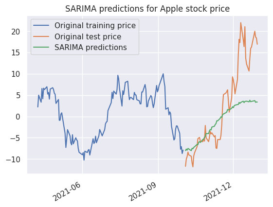
SARIMA#
1price_detrend = df_detrend["Close"]
Train test split#
1train_test_split_date = pd.Timestamp("2021-10-01")
2train, test = (
3    price_detrend[price_detrend.index <= train_test_split_date],
4    price_detrend[price_detrend.index > train_test_split_date],
5)
1model = sarimax(train)
2result = model.fit()
/home/runner/work/stock-analysis/stock-analysis/.venv/lib/python3.13/site-packages/statsmodels/tsa/base/tsa_model.py:473: ValueWarning: A date index has been provided, but it has no associated frequency information and so will be ignored when e.g. forecasting.
  self._init_dates(dates, freq)
/home/runner/work/stock-analysis/stock-analysis/.venv/lib/python3.13/site-packages/statsmodels/tsa/base/tsa_model.py:473: ValueWarning: A date index has been provided, but it has no associated frequency information and so will be ignored when e.g. forecasting.
  self._init_dates(dates, freq)
/home/runner/work/stock-analysis/stock-analysis/.venv/lib/python3.13/site-packages/statsmodels/base/model.py:607: ConvergenceWarning: Maximum Likelihood optimization failed to converge. Check mle_retvals
  warnings.warn("Maximum Likelihood optimization failed to "
1print(result.summary())
                               SARIMAX Results
==============================================================================
Dep. Variable:                  Close   No. Observations:                  694
Model:             SARIMAX(10, 0, 10)   Log Likelihood               -1419.635
Date:                Wed, 15 Oct 2025   AIC                           2881.270
Time:                        12:40:12   BIC                           2976.662
Sample:                             0   HQIC                          2918.160
                                - 694
Covariance Type:                  opg
==============================================================================
                 coef    std err          z      P>|z|      [0.025      0.975]
------------------------------------------------------------------------------
ar.L1          0.9860      0.112      8.769      0.000       0.766       1.206
ar.L2         -0.0215      0.091     -0.236      0.813      -0.200       0.157
ar.L3          0.0526      0.095      0.551      0.582      -0.134       0.240
ar.L4         -0.0071      0.093     -0.077      0.939      -0.189       0.174
ar.L5         -0.0374      0.081     -0.459      0.646      -0.197       0.122
ar.L6          0.0583      0.091      0.638      0.524      -0.121       0.237
ar.L7         -0.0317      0.091     -0.349      0.727      -0.210       0.146
ar.L8         -0.1617      0.083     -1.938      0.053      -0.325       0.002
ar.L9          0.9649      0.111      8.717      0.000       0.748       1.182
ar.L10        -0.8306      0.086     -9.655      0.000      -0.999      -0.662
ma.L1         -0.1299      0.119     -1.095      0.274      -0.362       0.103
ma.L2         -0.0127      0.093     -0.137      0.891      -0.195       0.169
ma.L3         -0.0716      0.090     -0.797      0.426      -0.248       0.105
ma.L4         -0.0788      0.104     -0.758      0.448      -0.283       0.125
ma.L5          0.0334      0.100      0.333      0.739      -0.163       0.230
ma.L6         -0.0906      0.091     -0.997      0.319      -0.269       0.088
ma.L7         -0.0072      0.106     -0.068      0.946      -0.215       0.201
ma.L8          0.1326      0.100      1.331      0.183      -0.063       0.328
ma.L9         -0.8112      0.103     -7.841      0.000      -1.014      -0.608
ma.L10         0.1090      0.043      2.560      0.010       0.026       0.192
sigma2         3.5329      0.138     25.571      0.000       3.262       3.804
===================================================================================
Ljung-Box (L1) (Q):                   0.00   Jarque-Bera (JB):               432.17
Prob(Q):                              0.95   Prob(JB):                         0.00
Heteroskedasticity (H):               6.79   Skew:                             0.01
Prob(H) (two-sided):                  0.00   Kurtosis:                         6.87
===================================================================================

Warnings:
[1] Covariance matrix calculated using the outer product of gradients (complex-step).
1forecast_steps = len(test)
2forecast = result.get_forecast(steps=forecast_steps)
3predicted_values = forecast.predicted_mean
/home/runner/work/stock-analysis/stock-analysis/.venv/lib/python3.13/site-packages/statsmodels/tsa/base/tsa_model.py:837: ValueWarning: No supported index is available. Prediction results will be given with an integer index beginning at `start`.
  return get_prediction_index(
/home/runner/work/stock-analysis/stock-analysis/.venv/lib/python3.13/site-packages/statsmodels/tsa/base/tsa_model.py:837: FutureWarning: No supported index is available. In the next version, calling this method in a model without a supported index will result in an exception.
  return get_prediction_index(
 1plot_n_days_prior_pred = 2 * forecast_steps
 2
 3plt.plot(train[-plot_n_days_prior_pred:], label="Original training price")
 4plt.plot(test, label="Original test price")
 5plt.plot(test.index, predicted_values, label="SARIMA predictions")
 6plt.title("SARIMA predictions for Apple stock price")
 7plt.legend()
 8
 9
10# Display limited number of date index
11plt.gca().xaxis.set_major_locator(mdates.MonthLocator(interval=3))
12# Rotate x-axis labels
13plt.gcf().autofmt_xdate()
14
15plt.show()
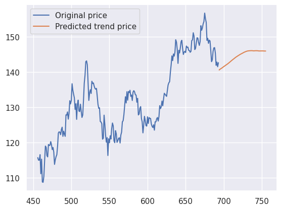
Prédiction du prix d’Apple à 2 mois#
Recomposons les prédictions du modèle SARIMA pour la stochasticité avec la tendance pour obtenir une prévision du cours d’Apple.
1original_data = load_stock_data(stock_name)
1# Get only close price
2original_price = original_data["Close"]
1# Train test split
2original_data_train, original_data_test = (
3    original_price[original_price.index <= train_test_split_date],
4    original_price[original_price.index > train_test_split_date],
5)
1# Drop time index in order to vanish weekend days issues
2original_data_train.reset_index(drop=True, inplace=True)
3original_data_test.reset_index(drop=True, inplace=True)
Tendance#
On reconstruit la tendance que l’on avait prédite par la méthode de la moyenne mobile.
1for i in range(forecast_steps):
2    rolling_mean = original_data_train.rolling(window=100, center=False).mean()
3    pred_trend = rolling_mean.iloc[-1]
4    pred_index = original_data_train.index[-1] + 1
5    original_data_train = pd.concat(
6        [original_data_train, pd.Series([pred_trend], index=[pred_index])]
7    )
1plt.plot(original_data_train.iloc[-300:-forecast_steps], label="Original price")
2plt.plot(
3    original_data_train.iloc[-forecast_steps:],
4    label="Predicted trend price",
5)
6plt.legend()
<matplotlib.legend.Legend at 0x7f3a93385310>
Saisonnalité et stochasticité#
1# Make SARIMA predicted values begin at zero
2predicted_values -= predicted_values.iloc[0]
1# Calculate trend + ARIMA
2add_components = original_data_train.iloc[-forecast_steps] + predicted_values
3
4# Put predicted data in train series set
5original_data_train.iloc[-forecast_steps:] = add_components
Evaluation de la prédiction#
1# Set index for test data i.e. actual data
2original_data_test.index = original_data_train.index[-forecast_steps:]
 1plt.plot(
 2    original_data_train.iloc[-200:-forecast_steps], color="blue", label="Original price"
 3)
 4plt.plot(
 5    original_data_train.iloc[-forecast_steps:],
 6    color="red",
 7    label="Predicted price with trend + seasonality + stochasticity",
 8)
 9plt.plot(original_data_test, color="green", label="Actual price")
10plt.legend()
<matplotlib.legend.Legend at 0x7f3a90169450>
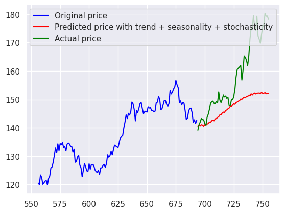
1y_true = original_data_test
2y_pred = original_data_train[-forecast_steps:]
1prediction_results_dict["SARIMA"] = compute_metrics(y_true, y_pred)
2prediction_results_dict["SARIMA"]
(10.698355198814452, 13.862575751530015)
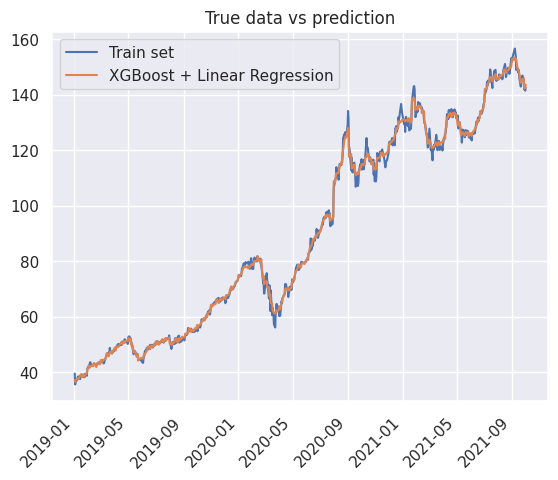
XGBoost#
Traitement des données#
1type(original_data)
pandas.core.frame.DataFrame
1train_start = pd.Timestamp("2019-01-01")
2train_end = pd.Timestamp("2021-10-01")
3
4df_train = original_data.loc[train_start:train_end].copy()
5df_test = original_data.loc[train_end:].copy()
1type(df_train)
2df_train["time_dummy"] = np.arange(len(df_train))
3df_train
| Open | High | Low | Close | Adj Close | Volume | time_dummy | |
|---|---|---|---|---|---|---|---|
| Date | |||||||
| 2019-01-02 | 38.722500 | 39.712502 | 38.557499 | 39.480000 | 37.943256 | 148158800 | 0 |
| 2019-01-03 | 35.994999 | 36.430000 | 35.500000 | 35.547501 | 34.163822 | 365248800 | 1 |
| 2019-01-04 | 36.132500 | 37.137501 | 35.950001 | 37.064999 | 35.622250 | 234428400 | 2 |
| 2019-01-07 | 37.174999 | 37.207500 | 36.474998 | 36.982498 | 35.542965 | 219111200 | 3 |
| 2019-01-08 | 37.389999 | 37.955002 | 37.130001 | 37.687500 | 36.220528 | 164101200 | 4 |
| ... | ... | ... | ... | ... | ... | ... | ... |
| 2021-09-27 | 145.470001 | 145.960007 | 143.820007 | 145.369995 | 143.707413 | 74150700 | 689 |
| 2021-09-28 | 143.250000 | 144.750000 | 141.690002 | 141.910004 | 140.286987 | 108972300 | 690 |
| 2021-09-29 | 142.470001 | 144.449997 | 142.029999 | 142.830002 | 141.196472 | 74602000 | 691 |
| 2021-09-30 | 143.660004 | 144.380005 | 141.279999 | 141.500000 | 139.881668 | 89056700 | 692 |
| 2021-10-01 | 141.899994 | 142.919998 | 139.110001 | 142.649994 | 141.018539 | 94639600 | 693 |
694 rows × 7 columns
1df_train["time_dummy"] = np.arange(len(df_train))
2df_test["time_dummy"] = np.arange(len(df_test)) + len(df_train)
3df_train["day"] = df_train.index.day
4df_test["day"] = df_test.index.day
1df_train["time_dummy"].tail()
Date
2021-09-27    689
2021-09-28    690
2021-09-29    691
2021-09-30    692
2021-10-01    693
Name: time_dummy, dtype: int64
1df_test["time_dummy"].head()
Date
2021-10-01    694
2021-10-04    695
2021-10-05    696
2021-10-06    697
2021-10-07    698
Name: time_dummy, dtype: int64
1x_col = ["time_dummy", "day"]
2y_col = ["Close"]
1x_train = df_train[x_col]
2y_train = df_train[y_col]
1x_test = df_test[x_col]
2y_test = df_test[y_col]
Apprentissage des modèles#
1lr = LinearRegression()
2lr.fit(x_train, y_train)
3y_residuals = y_train - lr.predict(x_train)
1xgb = xgboost.XGBRegressor(random_state=0, n_jobs=-2, colsample_bytree=0.3, max_depth=3)
2xgb.fit(x_train, y_residuals)
XGBRegressor(base_score=None, booster=None, callbacks=None,
             colsample_bylevel=None, colsample_bynode=None,
             colsample_bytree=0.3, device=None, early_stopping_rounds=None,
             enable_categorical=False, eval_metric=None, feature_types=None,
             feature_weights=None, gamma=None, grow_policy=None,
             importance_type=None, interaction_constraints=None,
             learning_rate=None, max_bin=None, max_cat_threshold=None,
             max_cat_to_onehot=None, max_delta_step=None, max_depth=3,
             max_leaves=None, min_child_weight=None, missing=nan,
             monotone_constraints=None, multi_strategy=None, n_estimators=None,
             n_jobs=-2, num_parallel_tree=None, ...)
In a Jupyter environment, please rerun this cell to show the HTML representation or trust the notebook. On GitHub, the HTML representation is unable to render, please try loading this page with nbviewer.org.
Parameters
| objective | 'reg:squarederror' | |
| base_score | None | |
| booster | None | |
| callbacks | None | |
| colsample_bylevel | None | |
| colsample_bynode | None | |
| colsample_bytree | 0.3 | |
| device | None | |
| early_stopping_rounds | None | |
| enable_categorical | False | |
| eval_metric | None | |
| feature_types | None | |
| feature_weights | None | |
| gamma | None | |
| grow_policy | None | |
| importance_type | None | |
| interaction_constraints | None | |
| learning_rate | None | |
| max_bin | None | |
| max_cat_threshold | None | |
| max_cat_to_onehot | None | |
| max_delta_step | None | |
| max_depth | 3 | |
| max_leaves | None | |
| min_child_weight | None | |
| missing | nan | |
| monotone_constraints | None | |
| multi_strategy | None | |
| n_estimators | None | |
| n_jobs | -2 | |
| num_parallel_tree | None | |
| random_state | 0 | |
| reg_alpha | None | |
| reg_lambda | None | |
| sampling_method | None | |
| scale_pos_weight | None | |
| subsample | None | |
| tree_method | None | |
| validate_parameters | None | |
| verbosity | None |
1y_pred_train = detrend_prediction(xgb, lr, x_train)
2y_pred_test = detrend_prediction(xgb, lr, x_test)
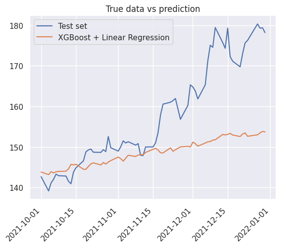
3prediction_results_dict["XGBoost"] = compute_metrics(y_test, y_pred_test)
4prediction_results_dict["XGBoost"]
(9.821550637003275, 13.252235166510234)
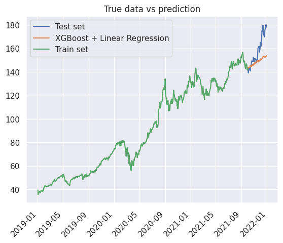
1_ = true_vs_prediction(
2    df_train["Close"],
3    y_pred_train,
4    true_label="Train set",
5    prediction_label="XGBoost + Linear Regression",
6)
1_ = true_vs_prediction(
2    df_test["Close"],
3    y_pred_test,
4    true_label="Test set",
5    prediction_label="XGBoost + Linear Regression",
6)
1true_vs_prediction(
2    df_test["Close"],
3    y_pred_test,
4    true_label="Test set",
5    prediction_label="XGBoost + Linear Regression",
6)
7plt.plot(df_train["Close"], label="Train set")
8plt.legend()
<matplotlib.legend.Legend at 0x7f3a900e6d50>
Extra Trees#
Apprentissage des modèles#
1et = ExtraTreesRegressor(random_state=0, n_jobs=-2)
2et.fit(x_train, y_residuals)
/home/runner/work/stock-analysis/stock-analysis/.venv/lib/python3.13/site-packages/sklearn/base.py:1365: DataConversionWarning: A column-vector y was passed when a 1d array was expected. Please change the shape of y to (n_samples,), for example using ravel().
  return fit_method(estimator, *args, **kwargs)
ExtraTreesRegressor(n_jobs=-2, random_state=0)In a Jupyter environment, please rerun this cell to show the HTML representation or trust the notebook.
On GitHub, the HTML representation is unable to render, please try loading this page with nbviewer.org.
Parameters
| n_estimators | 100 | |
| criterion | 'squared_error' | |
| max_depth | None | |
| min_samples_split | 2 | |
| min_samples_leaf | 1 | |
| min_weight_fraction_leaf | 0.0 | |
| max_features | 1.0 | |
| max_leaf_nodes | None | |
| min_impurity_decrease | 0.0 | |
| bootstrap | False | |
| oob_score | False | |
| n_jobs | -2 | |
| random_state | 0 | |
| verbose | 0 | |
| warm_start | False | |
| ccp_alpha | 0.0 | |
| max_samples | None | |
| monotonic_cst | None |
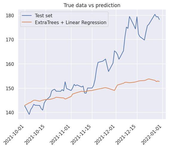
1y_pred_test = detrend_prediction(et, lr, x_test)
2prediction_results_dict["ExtraTrees"] = compute_metrics(y_test, y_pred_test)
3prediction_results_dict["ExtraTrees"]
(9.74557499696818, 13.20182282007082)
1_ = true_vs_prediction(
2    df_test["Close"],
3    y_pred_test,
4    true_label="Test set",
5    prediction_label="ExtraTrees + Linear Regression",
6)
SVM#
Apprentissage des modèles#
1svr = SVR()
2svr.fit(x_train, y_residuals)
/home/runner/work/stock-analysis/stock-analysis/.venv/lib/python3.13/site-packages/sklearn/utils/validation.py:1406: DataConversionWarning: A column-vector y was passed when a 1d array was expected. Please change the shape of y to (n_samples, ), for example using ravel().
  y = column_or_1d(y, warn=True)
SVR()In a Jupyter environment, please rerun this cell to show the HTML representation or trust the notebook.
On GitHub, the HTML representation is unable to render, please try loading this page with nbviewer.org.
Parameters
| kernel | 'rbf' | |
| degree | 3 | |
| gamma | 'scale' | |
| coef0 | 0.0 | |
| tol | 0.001 | |
| C | 1.0 | |
| epsilon | 0.1 | |
| shrinking | True | |
| cache_size | 200 | |
| verbose | False | |
| max_iter | -1 |
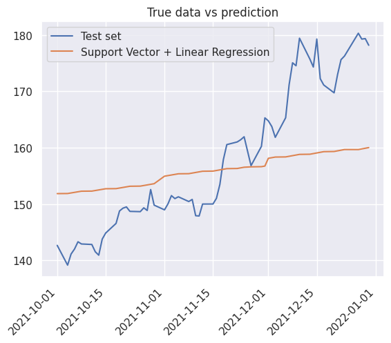
1y_pred_test = detrend_prediction(svr, lr, x_test)
2prediction_results_dict["Support Vector Machine"] = compute_metrics(y_test, y_pred_test)
3prediction_results_dict["Support Vector Machine"]
(8.73950426028892, 10.297525832287155)
1_ = true_vs_prediction(
2    df_test["Close"],
3    y_pred_test,
4    true_label="Test set",
5    prediction_label="Support Vector + Linear Regression",
6)
Prophet#
Pré-traitement pour Prophet#
 1x_train_prophet = pd.DataFrame(
 2    {
 3        "ds": x_train.index,
 4        "y": df_train["Close"].values,
 5    }
 6)
 7
 8x_test_prophet = pd.DataFrame(
 9    {
10        "ds": x_test.index,
11        "y": df_test["Close"].values,
12    }
13)
1x_test_prophet.head()
| ds | y | |
|---|---|---|
| 0 | 2021-10-01 | 142.649994 |
| 1 | 2021-10-04 | 139.139999 |
| 2 | 2021-10-05 | 141.110001 |
| 3 | 2021-10-06 | 142.000000 |
| 4 | 2021-10-07 | 143.289993 |
Prédiction#
Calcul de la prédiction#
1model = Prophet()
2model.fit(x_train_prophet)
12:40:14 - cmdstanpy - INFO - Chain [1] start processing
12:40:14 - cmdstanpy - INFO - Chain [1] done processing
<prophet.forecaster.Prophet at 0x7f3a974db8c0>
1forecast = model.predict(x_test_prophet)
2forecast[["ds", "yhat", "yhat_lower", "yhat_upper"]].tail()
| ds | yhat | yhat_lower | yhat_upper | |
|---|---|---|---|---|
| 58 | 2021-12-23 | 163.485849 | 157.429297 | 169.888856 |
| 59 | 2021-12-27 | 164.851525 | 158.423615 | 171.336812 |
| 60 | 2021-12-28 | 165.169482 | 158.395403 | 171.728886 |
| 61 | 2021-12-29 | 165.506546 | 159.233661 | 171.649162 |
| 62 | 2021-12-30 | 165.524170 | 159.169593 | 172.744326 |
1prediction_results_dict["Prophet"] = compute_metrics(
2    x_test_prophet["y"], forecast["yhat"]
3)
4prediction_results_dict["Prophet"]
(7.378329691676633, 9.228347960218333)
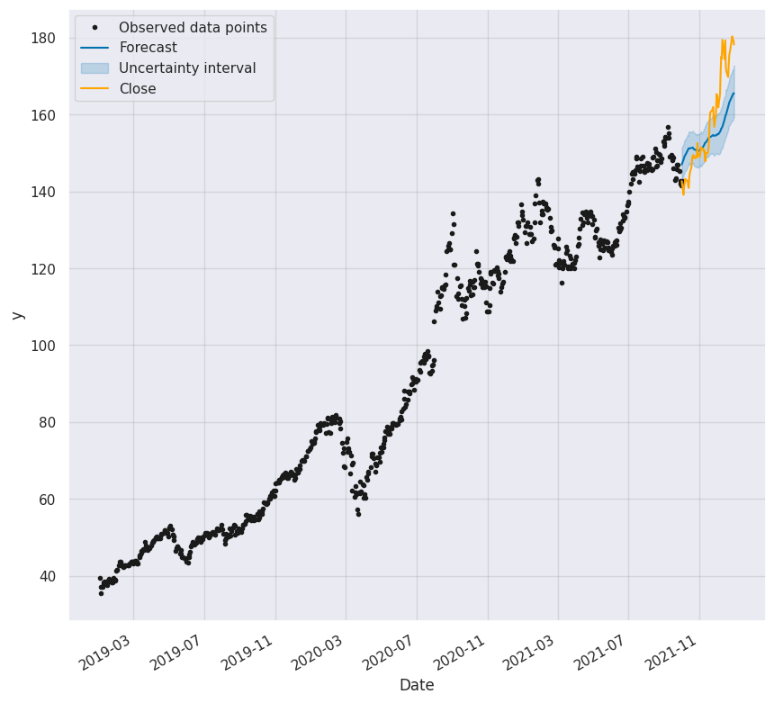
Affichage de la prédiction#
1fig, ax1 = plt.subplots(figsize=(10, 10))
2fig1 = model.plot(forecast, ax=ax1)
3# plt.scatter(forecast["ds"],df_test["Close"], color="orange", s=10, label="Close")
4df_test["Close"].plot(ax=ax1, color="orange")
5plt.legend()
/home/runner/work/stock-analysis/stock-analysis/.venv/lib/python3.13/site-packages/pandas/plotting/_matplotlib/core.py:981: UserWarning: This axis already has a converter set and is updating to a potentially incompatible converter
  return ax.plot(*args, **kwds)
<matplotlib.legend.Legend at 0x7f3a97526d50>
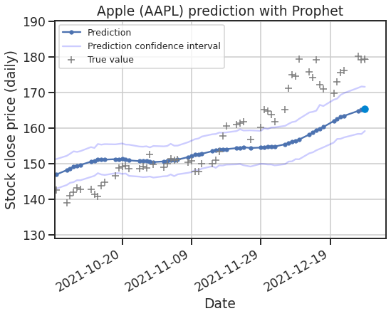
Animation#
1# Tailwind CSS colors
2sky600 = "#0084d1"
3orange600 = "#f54900"
1import matplotlib.animation as animation
2import matplotlib.dates as mdates
 1x = np.array(range(len(forecast["ds"])))
 2y_pred = forecast["yhat"]
 3y_lower = forecast["yhat_lower"]
 4y_upper = forecast["yhat_upper"]
 5x_dates = forecast["ds"]
 6x = mdates.date2num(x_dates)
 7
 8y_true = x_test_prophet["y"]
 9
10xmin, xmax, ymin, ymax = np.min(x), np.max(x), np.min(y_pred), np.max(y_pred)
1import seaborn as sns
2
3sns.set_theme(context="talk", style="ticks", rc={"axes.grid": True})
 1fig = plt.figure(figsize=(8, 6), dpi=75)
 2
 3plt.title("Apple (AAPL) prediction with Prophet")
 4plt.xlabel("Date")
 5plt.ylabel("Stock close price (daily)")
 6plt.gca().xaxis.set_major_formatter(mdates.DateFormatter("%Y-%m-%d"))
 7plt.gcf().autofmt_xdate()
 8
 9# initialise la figure
10(line_pred,) = plt.plot(
11    [],
12    [],
13    label="Prediction",
14    marker="o",
15    markersize=5,
16)
17(line_pred_upper,) = plt.plot(
18    [], [], label="Prediction confidence interval", color="blue", alpha=0.2
19)
20(line_pred_lower,) = plt.plot([], [], color="blue", alpha=0.2)
21(line_true,) = plt.plot(
22    [],
23    [],
24    label="True value",
25    ls="none",
26    marker="+",
27    markersize=10,
28    color="gray",
29    markeredgewidth=1.5,
30)
31
32(point_pred,) = plt.plot([], [], ls="none", marker="o", color=sky600)
33(point_true,) = plt.plot([], [], ls="none", marker="+", markersize=10, color="gray")
34
35plt.legend(loc="upper left", fontsize=12)
36
37plt.xlim(xmin, xmax)
38plt.ylim(ymin, ymax)
39
40padding_x = 5
41padding_y = 10
42
43
44def animate(i: int):
45    x_data = x[: i + 1]
46    y_data = (y_pred[: i + 1], y_true[: i + 1], y_upper[: i + 1], y_lower[: i + 1])
47    xmin, xmax, ymin, ymax = (
48        np.min(x_data) - padding_x / 10,
49        np.max(x_data) + padding_x,
50        np.min(np.concatenate(y_data)) - padding_y,
51        np.max(np.concatenate(y_data)) + padding_y,
52    )
53    plt.xlim(xmin, xmax)
54    plt.ylim(ymin, ymax)
55
56    point_pred.set_data(x[i - 1 : i], y_pred[i - 1 : i])
57    line_pred.set_data(x[:i], y_pred[:i])
58    line_pred_upper.set_data(x[:i], y_upper[:i])
59    line_pred_lower.set_data(x[:i], y_lower[:i])
60
61    point_true.set_data(x[i - 1 : i], y_true[i - 1 : i])
62    line_true.set_data(x[:i], y_true[:i])
63
64    return line_pred, line_true
65
66
67ani = animation.FuncAnimation(
68    fig, animate, frames=len(x), interval=1, blit=True, repeat=False
69)
70ani.save("assets/img/prophet-prediction.gif")
MovieWriter ffmpeg unavailable; using Pillow instead.
1plt.rcParams["axes.prop_cycle"].by_key()["color"]
[(0.2980392156862745, 0.4470588235294118, 0.6901960784313725),
 (0.8666666666666667, 0.5176470588235295, 0.3215686274509804),
 (0.3333333333333333, 0.6588235294117647, 0.40784313725490196),
 (0.7686274509803922, 0.3058823529411765, 0.3215686274509804),
 (0.5058823529411764, 0.4470588235294118, 0.7019607843137254),
 (0.5764705882352941, 0.47058823529411764, 0.3764705882352941),
 (0.8549019607843137, 0.5450980392156862, 0.7647058823529411),
 (0.5490196078431373, 0.5490196078431373, 0.5490196078431373),
 (0.8, 0.7254901960784313, 0.4549019607843137),
 (0.39215686274509803, 0.7098039215686275, 0.803921568627451)]
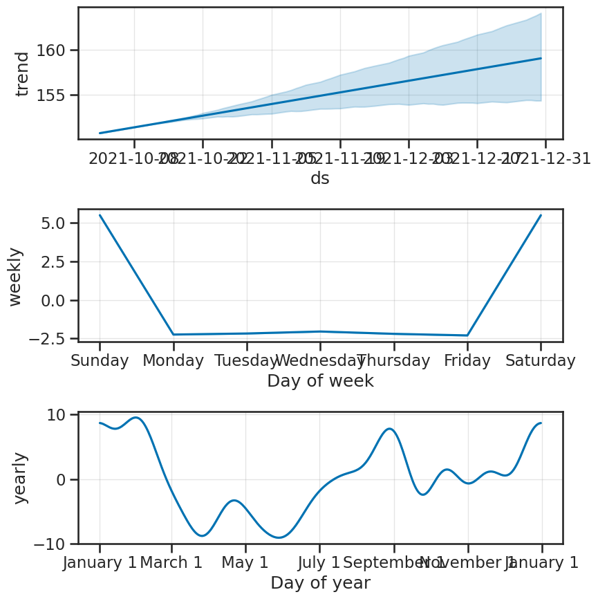
Décomposition#
1fig2 = model.plot_components(forecast)
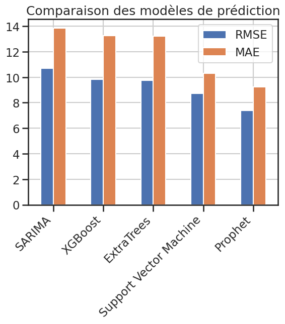
Comparaison des modèles#
1prediction_results_df = pd.DataFrame(prediction_results_dict).T
2prediction_results_df.columns = ["RMSE", "MAE"]
3# prediction_results_df
1prediction_results_df.plot(kind="bar")
2plt.title("Comparaison des modèles de prédiction")
3
4plt.xticks(rotation=45, ha="right")
(array([0, 1, 2, 3, 4]),
 [Text(0, 0, 'SARIMA'),
  Text(1, 0, 'XGBoost'),
  Text(2, 0, 'ExtraTrees'),
  Text(3, 0, 'Support Vector Machine'),
  Text(4, 0, 'Prophet')])
1# print(prediction_results_df.to_markdown())
Tableau. Comparaison des modèles de prédiction
RMSE |
MAE |
Graphiquement |
|
|---|---|---|---|
ARMA |
17.3524 |
14.9797 |
✅ |
SARIMA |
13.6817 |
11.6047 |
✅ |
XGBoost |
13.2914 |
9.85264 |
✅ |
ExtraTrees |
13.2018 |
9.74557 |
✅ |
Support Vector Machine |
10.2975 |
8.7395 |
❌ |
Prophet |
8.97155 |
7.26206 |
✅ |
Meilleur modèle : Prophet