 1import matplotlib.pyplot as plt
 2import numpy as np
 3import pandas as pd
 4import seaborn as sns
 5from src.code.simulation.galton_watson import SimulateurGaltonWatson
 6from src.code.simulation.probability_distributions import (
 7    create_distributions,
 8    create_distributions_df,
 9)
10from src.code.simulation.utils import test_loi_exponentielle
11from src.code.simulation.yaglom import simulation_yaglom_toutes_lois
12from src.config.config import seed
13from src.utils.utils import init_notebook
1init_notebook(seed)
Théorème de Yaglom#
Mise au propre Yaglom#
1distributions = create_distributions()
1alpha = 0.05
2nb_processus = 30_000
3taille_pas = 2
4nb_repetitions = 100
1p_value_dict, ks_dict, lambda_dict = simulation_yaglom_toutes_lois(
2    distributions,
3    nb_processus,
4    taille_pas,
5    nb_repetitions,
6)
---------------------------------------------------------------------------
KeyboardInterrupt                         Traceback (most recent call last)
Cell In[5], line 1
----> 1 p_value_dict, ks_dict, lambda_dict = simulation_yaglom_toutes_lois(
      2     distributions,
      3     nb_processus,
      4     taille_pas,
      5     nb_repetitions,
      6 )

File ~/work/epidemic-simulation/epidemic-simulation/src/code/simulation/yaglom.py:85, in simulation_yaglom_toutes_lois(distributions, nb_processus, taille_pas, nb_repetitions)
     82 lambda_dict: dict[str, list[float]] = {}
     84 for nom_loi, loi in distributions.items():
---> 85     p_value, ks, lambda_ = simulation_yaglom(
     86         loi,
     87         nb_processus=nb_processus,
     88         taille_pas=taille_pas,
     89         nb_repetitions=nb_repetitions,
     90     )
     92     p_value_dict[nom_loi] = p_value
     93     ks_dict[nom_loi] = ks

File ~/work/epidemic-simulation/epidemic-simulation/src/code/simulation/yaglom.py:48, in simulation_yaglom(loi, nb_processus, taille_pas, nb_repetitions, taille_echantillon, affichage)
     45 sim = SimulateurGaltonWatson(loi, nb_processus=nb_processus)
     47 for i in range(nb_repetitions):
---> 48     sim.simule(nb_epoques=taille_pas)
     49     sim.retire_processus_eteints()
     51     zn_sur_n = sim.get_zn_sur_n()

File ~/work/epidemic-simulation/epidemic-simulation/src/code/simulation/galton_watson.py:207, in SimulateurGaltonWatson.simule(self, nb_epoques)
    205 def simule(self, nb_epoques: int = 10) -> None:
    206     for i in range(self.nb_processus):
--> 207         self.simulations[i].simule(nb_epoques)

File ~/work/epidemic-simulation/epidemic-simulation/src/code/simulation/galton_watson.py:60, in GaltonWatson.simule(self, nb_epoques)
     57 epoque_actuelle = 0
     59 while epoque_actuelle < nb_epoques and self.nb_descendants > 0:
---> 60     liste_descendants = self.loi.rvs(size=self.nb_descendants)
     61     self.liste_descendants.append(liste_descendants)
     63     self.nb_descendants = np.sum(liste_descendants)

File ~/work/epidemic-simulation/epidemic-simulation/.venv/lib/python3.14/site-packages/scipy/stats/_distn_infrastructure.py:544, in rv_frozen.rvs(self, size, random_state)
    542 kwds = self.kwds.copy()
    543 kwds.update({'size': size, 'random_state': random_state})
--> 544 return self.dist.rvs(*self.args, **kwds)

File ~/work/epidemic-simulation/epidemic-simulation/.venv/lib/python3.14/site-packages/scipy/stats/_distn_infrastructure.py:3501, in rv_discrete.rvs(self, *args, **kwargs)
   3472 """Random variates of given type.
   3473
   3474 Parameters
   (...)   3498
   3499 """
   3500 kwargs['discrete'] = True
-> 3501 return super().rvs(*args, **kwargs)

File ~/work/epidemic-simulation/epidemic-simulation/.venv/lib/python3.14/site-packages/scipy/stats/_distn_infrastructure.py:1113, in rv_generic.rvs(self, *args, **kwds)
   1111 args, loc, scale, size = self._parse_args_rvs(*args, **kwds)
   1112 cond = logical_and(self._argcheck(*args), (scale >= 0))
-> 1113 if not np.all(cond):
   1114     message = ("Domain error in arguments. The `scale` parameter must "
   1115                "be positive for all distributions, and many "
   1116                "distributions have restrictions on shape parameters. "
   1117                f"Please see the `scipy.stats.{self.name}` "
   1118                "documentation for details.")
   1119     raise ValueError(message)

File ~/work/epidemic-simulation/epidemic-simulation/.venv/lib/python3.14/site-packages/numpy/_core/fromnumeric.py:2634, in all(a, axis, out, keepdims, where)
   2548 @array_function_dispatch(_all_dispatcher)
   2549 def all(a, axis=None, out=None, keepdims=np._NoValue, *, where=np._NoValue):
   2550     """
   2551     Test whether all array elements along a given axis evaluate to True.
   2552
   (...)   2632
   2633     """
-> 2634     return _wrapreduction_any_all(a, np.logical_and, 'all', axis, out,
   2635                                   keepdims=keepdims, where=where)

File ~/work/epidemic-simulation/epidemic-simulation/.venv/lib/python3.14/site-packages/numpy/_core/fromnumeric.py:97, in _wrapreduction_any_all(obj, ufunc, method, axis, out, **kwargs)
     95         pass
     96     else:
---> 97         return reduction(axis=axis, out=out, **passkwargs)
     99 return ufunc.reduce(obj, axis, bool, out, **passkwargs)

File ~/work/epidemic-simulation/epidemic-simulation/.venv/lib/python3.14/site-packages/numpy/_core/_methods.py:70, in _all(a, axis, dtype, out, keepdims, where)
     68 # Parsing keyword arguments is currently fairly slow, so avoid it for now
     69 if where is True:
---> 70     return umr_all(a, axis, dtype, out, keepdims)
     71 return umr_all(a, axis, dtype, out, keepdims, where=where)

KeyboardInterrupt:
1p_value_df = pd.DataFrame(p_value_dict)
2ks_df = pd.DataFrame(ks_dict)
3lambda_df = pd.DataFrame(lambda_dict)
1p_value_df.to_csv("data/results/p-value-evolution.csv", index=False)
2ks_df.to_csv("data/results/ks-evolution.csv", index=False)
3lambda_df.to_csv("data/results/lambda-evolution.csv", index=False)
1p_value_df = pd.read_csv("data/results/p-value-evolution.csv")
2ks_df = pd.read_csv("data/results/ks-evolution.csv")
3lambda_df = pd.read_csv("data/results/lambda-evolution.csv")
1distributions_df = create_distributions_df()
1lambda_array = np.array(distributions_df["Lambda théorique loi exponentielle Z_n / n"])
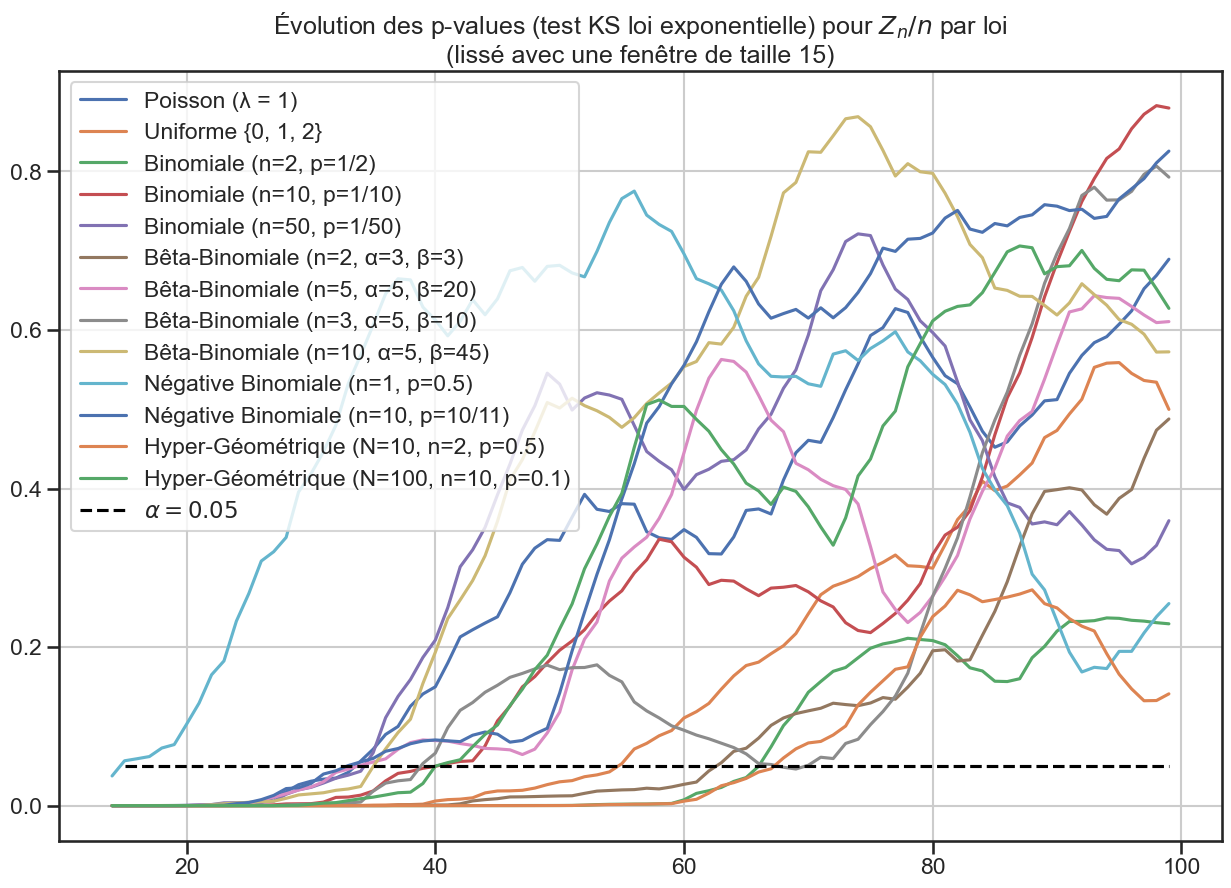
Graphiques#
p-values#
Toutes les lois de reproduction#
 1periode_lissage = 15
 2
 3p_value_df.rolling(window=periode_lissage).mean().plot(figsize=(15, 10))
 4plt.title(
 5    "Évolution des p-values (test KS loi exponentielle) pour $Z_n / n$ par loi"
 6    f"\n(lissé avec une fenêtre de taille {periode_lissage})",
 7)
 8plt.plot(
 9    list(range(periode_lissage, nb_repetitions)),
10    [alpha for _ in range(periode_lissage, nb_repetitions)],
11    label=r"$\alpha = 0.05$",
12    color="black",
13    linestyle="dashed",
14)
15plt.legend()
16plt.savefig("assets/img/p-values-evolution-all-laws.png")
17plt.savefig("assets/img/p-values-evolution-all-laws.svg")
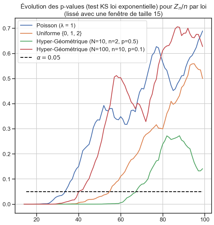
Lois de reproduction groupées#
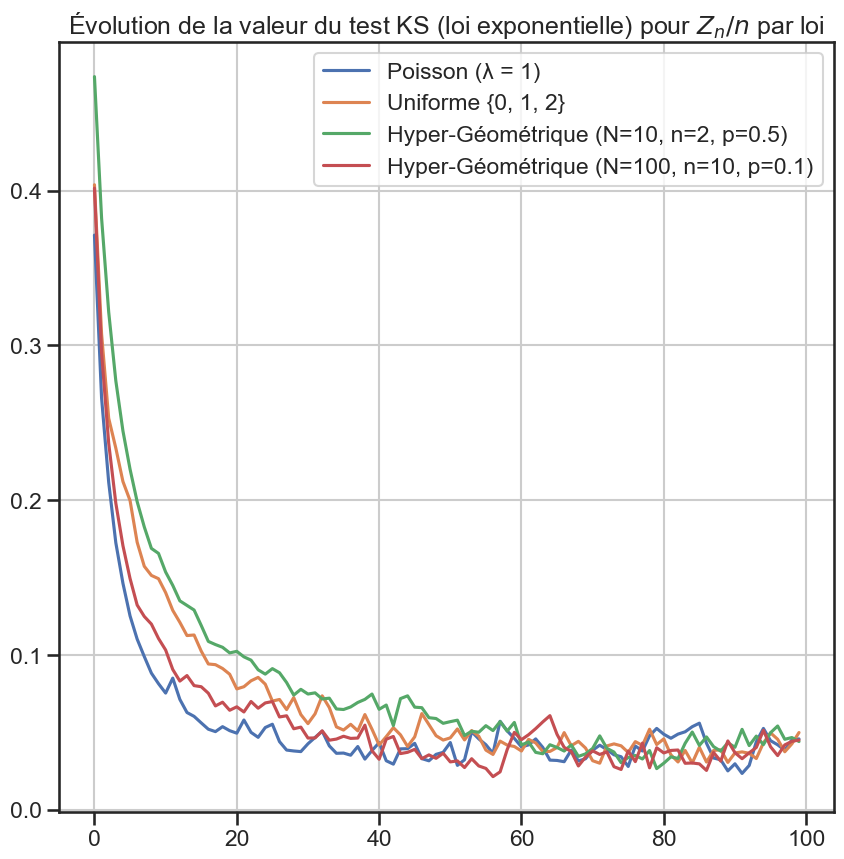
1groupe1 = [
2 "Poisson (λ = 1)",
3 "Uniforme {0, 1, 2}",
4 "Hyper-Géométrique (N=10, n=2, p=0.5)",
5 "Hyper-Géométrique (N=100, n=10, p=0.1)",
6]
7
8groupe2 = [
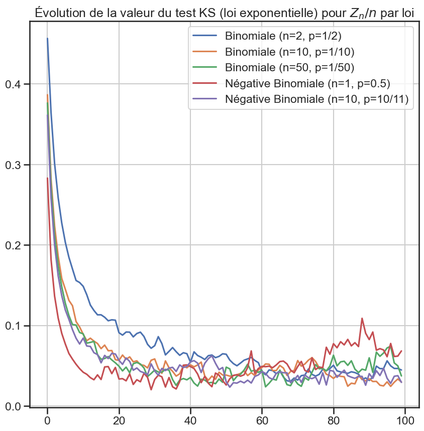
9 "Binomiale (n=2, p=1/2)",
10 "Binomiale (n=10, p=1/10)",
11 "Binomiale (n=50, p=1/50)",
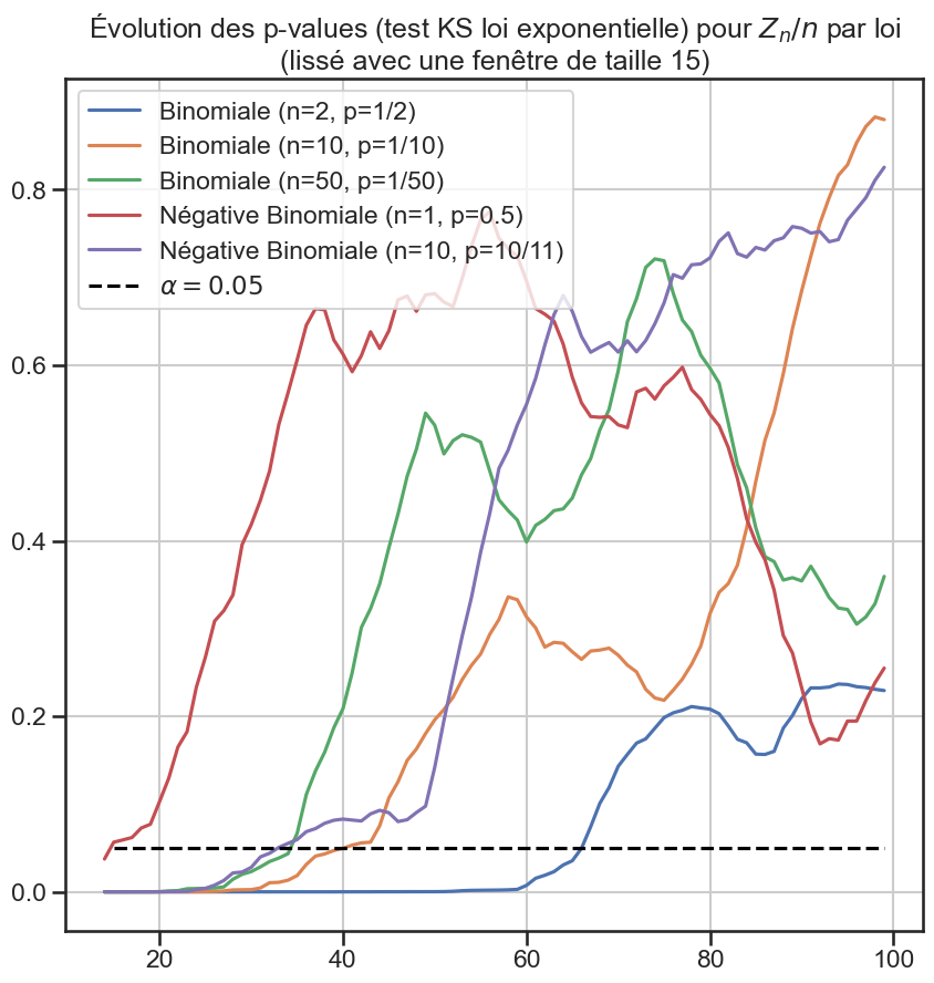
12 "Négative Binomiale (n=1, p=0.5)",
13 "Négative Binomiale (n=10, p=10/11)",
14]
15
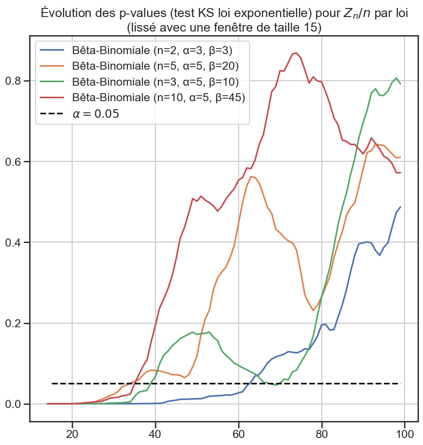
16groupe3 = [
17 "Bêta-Binomiale (n=2, α=3, β=3)",
18 "Bêta-Binomiale (n=5, α=5, β=20)",
19 "Bêta-Binomiale (n=3, α=5, β=10)",
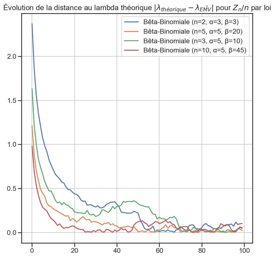
20 "Bêta-Binomiale (n=10, α=5, β=45)",
21]
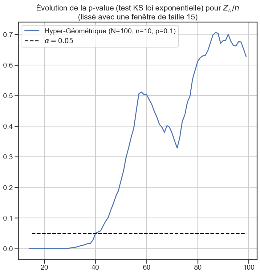
 1periode_lissage = 15
 2
 3p_value_df["Hyper-Géométrique (N=100, n=10, p=0.1)"].rolling(
 4    window=periode_lissage,
 5).mean().plot(figsize=(10, 10))
 6
 7plt.title(
 8    "Évolution de la p-value (test KS loi exponentielle) pour $Z_n / n$"
 9    f"\n(lissé avec une fenêtre de taille {periode_lissage})",
10)
11plt.plot(
12    list(range(periode_lissage, nb_repetitions)),
13    [alpha for _ in range(periode_lissage, nb_repetitions)],
14    label=r"$\alpha = 0.05$",
15    color="black",
16    linestyle="dashed",
17)
18plt.legend()
19plt.savefig("data/plots/evolution/p-value-hypergeom.png")
 1periode_lissage = 15
 2
 3p_value_df[groupe1].rolling(window=periode_lissage).mean().plot(figsize=(10, 10))
 4
 5plt.title(
 6    "Évolution des p-values (test KS loi exponentielle) pour $Z_n / n$ par loi"
 7    f"\n(lissé avec une fenêtre de taille {periode_lissage})",
 8)
 9plt.plot(
10    list(range(periode_lissage, nb_repetitions)),
11    [alpha for _ in range(periode_lissage, nb_repetitions)],
12    label=r"$\alpha = 0.05$",
13    color="black",
14    linestyle="dashed",
15)
16plt.legend()
17plt.savefig("data/plots/evolution/p-value-group1.png")
 1periode_lissage = 15
 2
 3p_value_df[groupe2].rolling(window=periode_lissage).mean().plot(figsize=(10, 10))
 4
 5plt.title(
 6    "Évolution des p-values (test KS loi exponentielle) pour $Z_n / n$ par loi"
 7    f"\n(lissé avec une fenêtre de taille {periode_lissage})",
 8)
 9plt.plot(
10    list(range(periode_lissage, nb_repetitions)),
11    [alpha for _ in range(periode_lissage, nb_repetitions)],
12    label=r"$\alpha = 0.05$",
13    color="black",
14    linestyle="dashed",
15)
16plt.legend()
17
18plt.savefig("data/plots/evolution/p-value-group2.png")
 1periode_lissage = 15
 2
 3p_value_df[groupe3].rolling(window=periode_lissage).mean().plot(figsize=(10, 10))
 4
 5plt.title(
 6    "Évolution des p-values (test KS loi exponentielle) pour $Z_n / n$ par loi"
 7    f"\n(lissé avec une fenêtre de taille {periode_lissage})",
 8)
 9plt.plot(
10    list(range(periode_lissage, nb_repetitions)),
11    [alpha for _ in range(periode_lissage, nb_repetitions)],
12    label=r"$\alpha = 0.05$",
13    color="black",
14    linestyle="dashed",
15)
16plt.legend()
17
18plt.savefig("data/plots/evolution/p-value-group3.png")
Statistique KS#
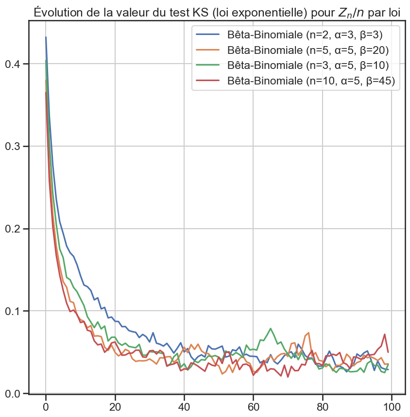
 1for group_name, group in (
 2    ("group1", groupe1),
 3    ("group2", groupe2),
 4    ("group3", groupe3),
 5):
 6    ks_df[group].plot(figsize=(10, 10))
 7
 8    plt.title(
 9        "Évolution de la valeur du test KS (loi exponentielle) pour $Z_n / n$ par loi",
10    )
11
12    plt.savefig(f"data/plots/evolution/ks-{group_name}.png")
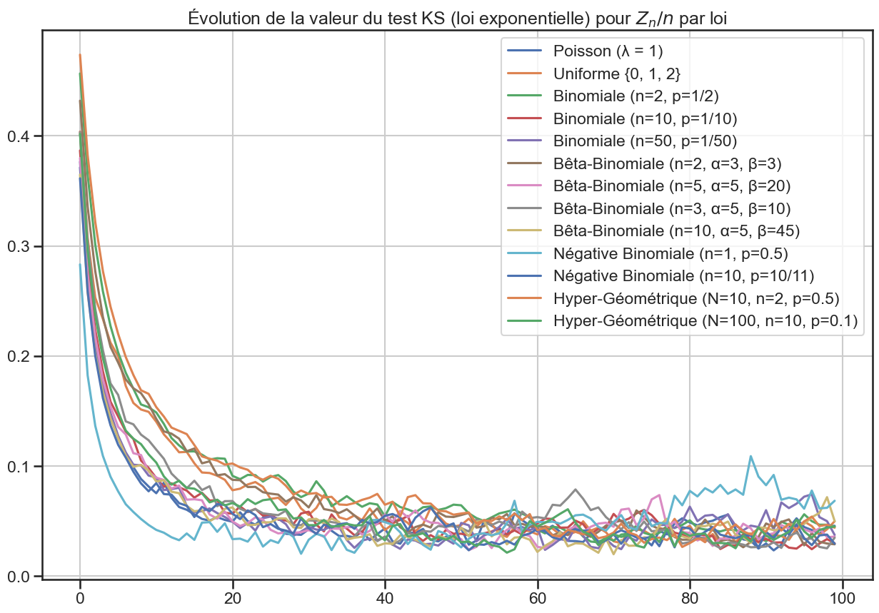
1ks_df.plot(figsize=(15, 10))
2
3plt.title(
4    "Évolution de la valeur du test KS (loi exponentielle) pour $Z_n / n$ par loi",
5)
6
7plt.savefig("data/plots/evolution/ks-all.png")
Distance au lambda théorique#
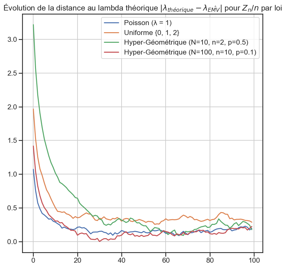
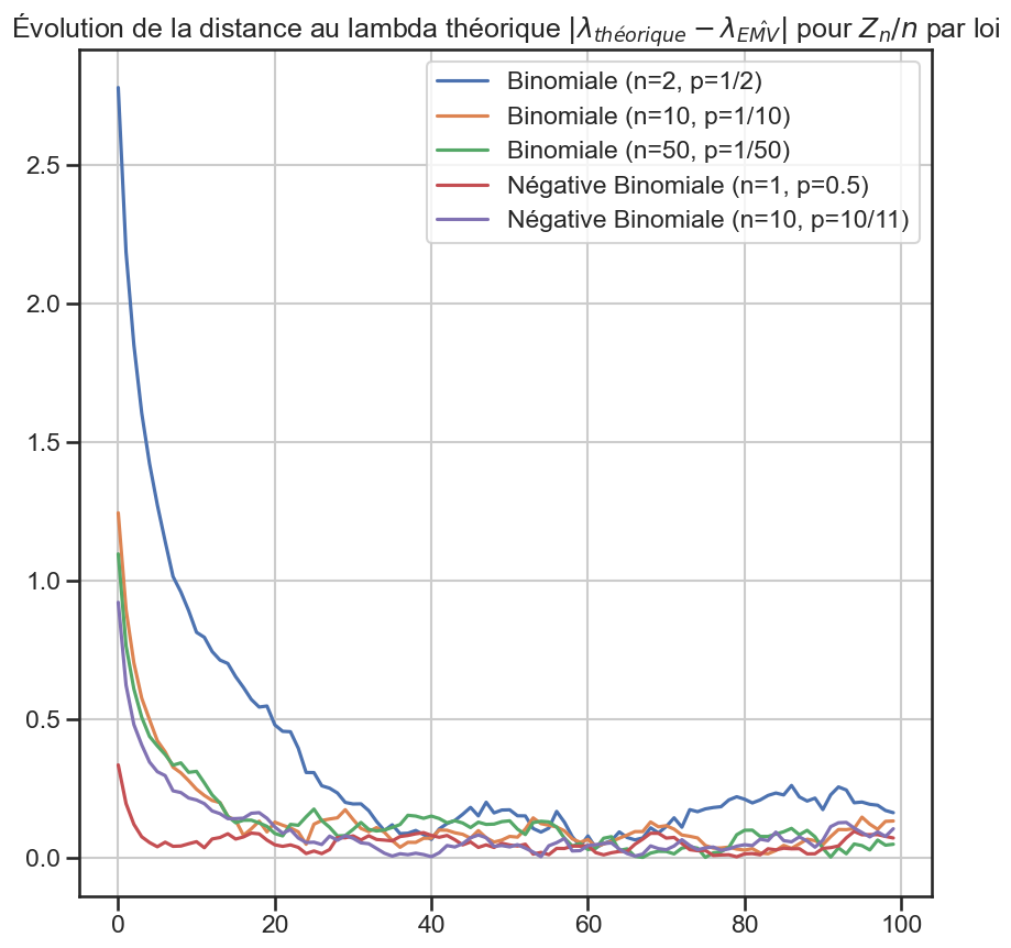
 1for group_name, group in (
 2    ("group1", groupe1),
 3    ("group2", groupe2),
 4    ("group3", groupe3),
 5):
 6    index = [list(lambda_df.columns).index(group[i]) for i in range(len(group))]
 7
 8    abs(lambda_df[group] - lambda_array[index]).plot(figsize=(10, 10))
 9
10    plt.title(
11        r"Évolution de la distance au lambda théorique $|\lambda_{théorique} - \lambda_{\hat{EMV}}|$ pour $Z_n / n$ par loi",
12    )
13
14    plt.savefig(f"data/plots/evolution/lambda-distance-{group_name}.png")
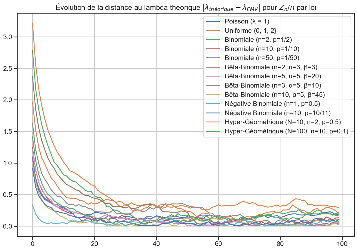
1abs(lambda_df - lambda_array).plot(figsize=(15, 10))
2
3plt.title(
4    r"Évolution de la distance au lambda théorique $|\lambda_{théorique} - \lambda_{\hat{EMV}}|$ pour $Z_n / n$ par loi",
5)
6
7plt.savefig("data/plots/evolution/lambda-distance-all.png")
Évolution de la distribution#
 1sim = SimulateurGaltonWatson(
 2    distributions["Hyper-Géométrique (N=10, n=2, p=0.5)"],
 3    nb_processus=10_000,
 4)
 5taille_pas = 5
 6nb_repetitions = 10
 7taille_echantillon = 100
 8
 9for i in range(nb_repetitions):
10    sim.simule(nb_epoques=taille_pas)
11    sim.retire_processus_eteints()
12
13    zn_sur_n = sim.get_zn_sur_n()
14    zn_sur_n_sample = zn_sur_n[taille_echantillon:]
15
16    plt.title(
17        r"Distribution des $\dfrac{Z_n}{n}$ à l'époque $n = "
18        + str((i + 1) * taille_pas)
19        + "$",
20    )
21    sns.histplot(zn_sur_n_sample, stat="density")
22    plt.savefig(f"data/results/distribution/hyper-geo-{(i + 1) * taille_pas}.png")
23    plt.show()
24
25    p_value, statistique_ks = test_loi_exponentielle(zn_sur_n)
26    print(f"{p_value = }")
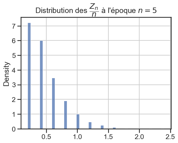
p_value = 0.0
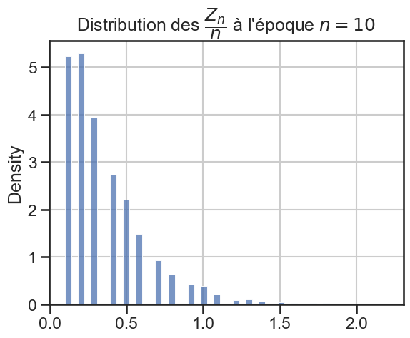
p_value = 9.622011434558595e-152
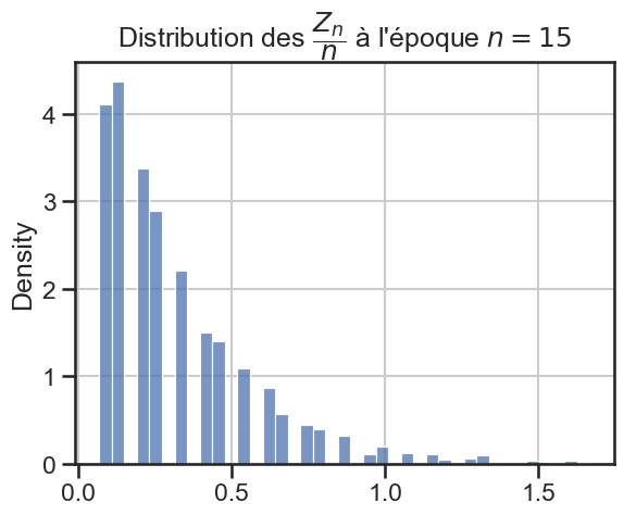
p_value = 2.827435930932723e-70
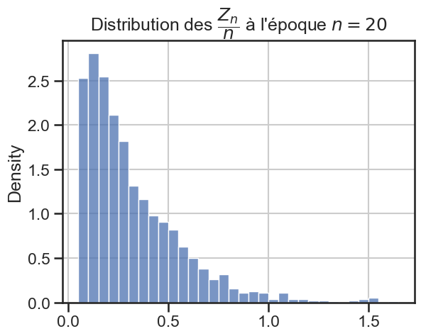
p_value = 2.8210546622397323e-39
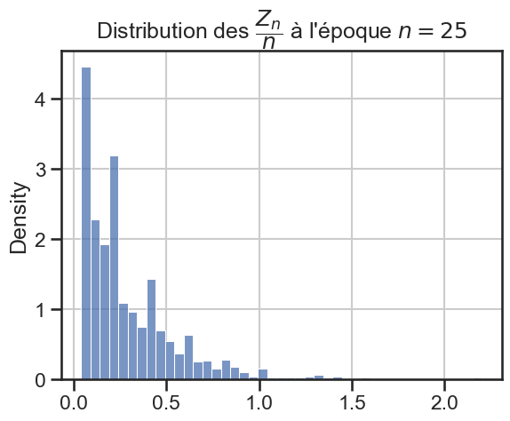
p_value = 3.2216117932465623e-24
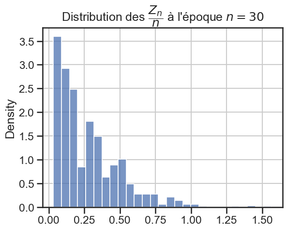
p_value = 7.887052073352042e-20
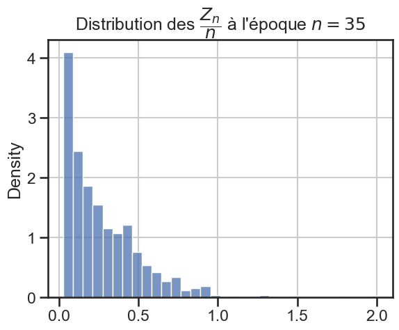
p_value = 3.461167774975927e-12
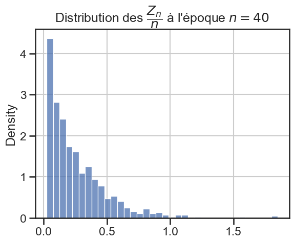
p_value = 1.7994986428624622e-12
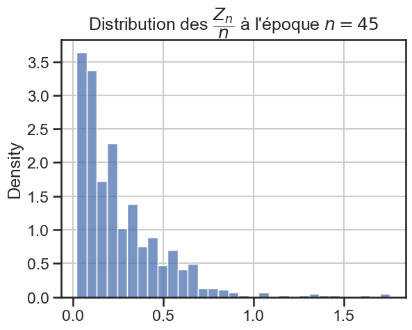
p_value = 7.08994488987903e-08
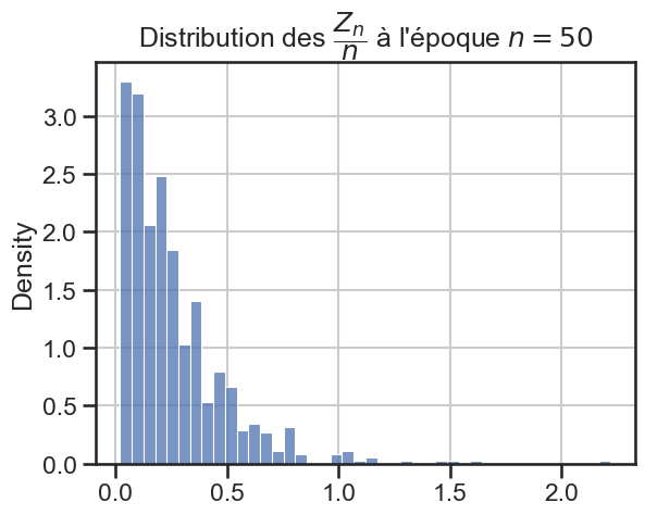
p_value = 3.728747180083857e-08
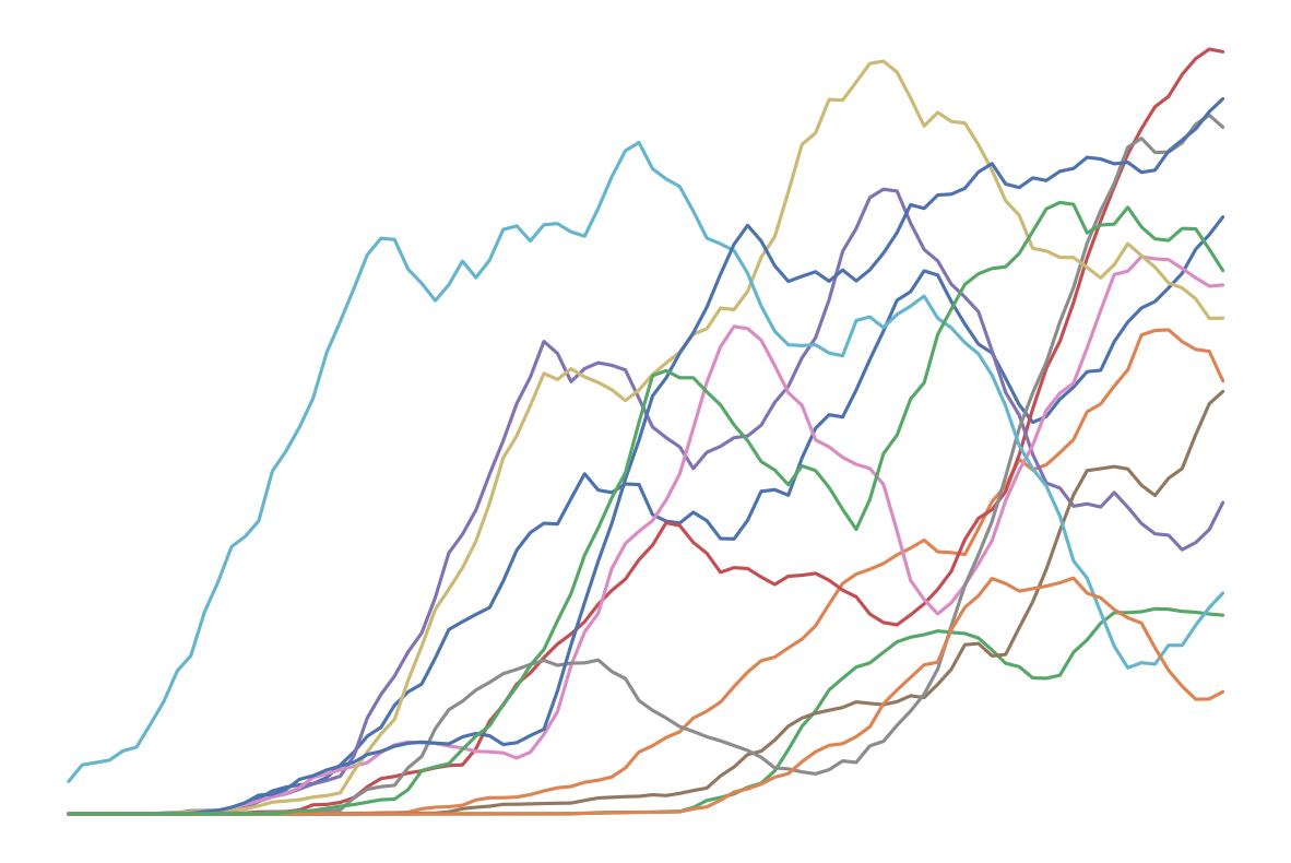
Graphique transparent (pour le style)#
 1periode_lissage = 15
 2p_value_df.rolling(window=periode_lissage).mean().plot(figsize=(15, 10), legend=None)
 3
 4plt.plot(
 5    list(range(periode_lissage, nb_repetitions)),
 6    [alpha for _ in range(periode_lissage, nb_repetitions)],
 7    label=r"$\alpha = 0.05$",
 8    color="black",
 9    linestyle="dashed",
10)
11plt.grid(False)
12
13# Remove both x and y axes
14plt.axis("off")
15# Hide major ticks and labels on the x-axis
16plt.tick_params(axis="x", which="major", length=0, labelbottom=False)
17
18# Hide major ticks and labels on the y-axis
19plt.tick_params(axis="y", which="major", length=0, labelleft=False)
20# plt.savefig("assets/img/p-values-evolution-all-laws.svg")
21
22plt.savefig("assets/img/p-values-evolution-all-laws-transparent.png", transparent=True)